Analysing data you already have

Start from trial-level data

One row per trial. The only columns that matter are stimulus and response; a participant column lets you split a sample.

participant  trial stimulus response
        p01      1    a2/b2    a2/b1
        p01      2    a2/b1    a2/b1
        p01      3    a2/b2    a2/b2
        p01      4    a1/b2    a1/b2
        p01      5    a2/b2    a1/b1
        p01      6    a2/b2    a2/b2

Levels are written as a1/b2 — the level on each dimension, separated by a character you choose. Order carries meaning that a bare label cannot express, so the packages will not guess it: you say which levels belong to which factor and they do the placement.

import pandas as pd, grintools as gt

trials = pd.read_csv("my_experiment.csv")
one = trials[trials.participant == "p01"]

ci = gt.to_confusion(
    one, long=True,
    factor_a=("a1", "a2"),
    factor_b=("b1", "b2"),
    sep="/",
)
print(ci.counts)

library(grin)

trials <- read.csv("my_experiment.csv")
one <- trials[trials$participant == "p01", ]

ci <- grin_to_confusion(
  one,
  factor_a = c("a1", "a2"),
  factor_b = c("b1", "b2"),
  sep = "/"
)
print(ci$counts)

[[29  2  3  6]
 [ 1 32  0  2]
 [ 2  3 36  4]
 [ 2  6  3 29]]

Rows are stimuli and columns responses, both ordered A1B1, A1B2, A2B1, A2B2. If your file already has a 4×4 matrix in that order, skip this step and pass it straight in.

Fit it

One call, well under a millisecond.

fit, con = gt.infer(ci.counts)
print(fit.summary())

fit <- grin_infer(ci$counts)
print(fit)

GRIN inference (onnx)
----------------------------------------------
  zx_0    = -0.85  +/- 0.27   [90% -1.30, -0.41]
  zx_1    = -1.57  +/- 0.38   [90% -2.19, -0.94]
  zx_2    = +1.18  +/- 0.29   [90% +0.69, +1.66]
  zx_3    = +0.82  +/- 0.25   [90% +0.40, +1.23]
  zy_0    = -0.90  +/- 0.25   [90% -1.31, -0.48]
  zy_1    = +1.87  +/- 0.37   [90% +1.25, +2.49]
  zy_2    = -0.93  +/- 0.25   [90% -1.34, -0.51]
  zy_3    = +1.24  +/- 0.26   [90% +0.80, +1.67]
  rho_0   = +0.55  +/- 0.32   [90% +0.02, +1.09]
  rho_1   = +0.14  +/- 0.55   [90% -0.76, +1.05]
  rho_2   = -0.21  +/- 0.40   [90% -0.87, +0.44]
  rho_3   = +0.26  +/- 0.42   [90% -0.43, +0.95]
----------------------------------------------
  componentwise modal structure : free + !PS(A) + PS(B)
  intervals are the network's own; pass calibrated=True for
  width-corrected intervals (see the package documentation)

Note rho_0: the interval runs past 1.0. The point estimate of a correlation is always valid, but the shipped interval is a symmetric Gaussian one in parameter space and is not clipped to (−1, 1). Read such an interval as “everything up to the boundary”.

Read the constructs

for k, dk in (("p_PI", "decision_PI"),
              ("p_sep_A", "decision_sep_A"),
              ("p_sep_B", "decision_sep_B")):
    print(k, con[k], con[dk])

con <- fit$constructs
con$p_PI;    con$decision_PI
con$p_sep_A; con$decision_sep_A
con$p_sep_B; con$decision_sep_B

p_PI      0.024    decision: against
p_sep_A   0.292    decision: undecided
p_sep_B   0.550    decision: undecided

The direction-explicit decision is the useful part. Here independence is clearly rejected, but neither separability call is far enough from one half to report as a finding — which is the honest answer, not a failure.

Report it

The perceptual space is the conventional way to present a GRT result. All four plots come straight off the fitted object and default to a greyscale-safe style.

from grintools.plot import (plot_space, plot_params,
                            plot_constructs, plot_diagnostics)

plot_space(fit)

plot_space(fit)

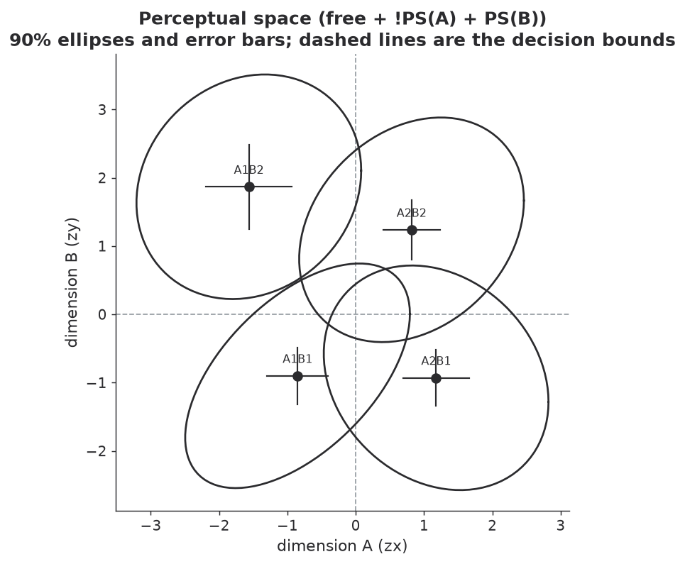
plot_params(fit)

plot_params(fit)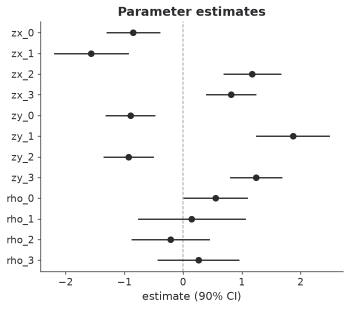

plot_constructs(fit, con)

plot_constructs(fit, con)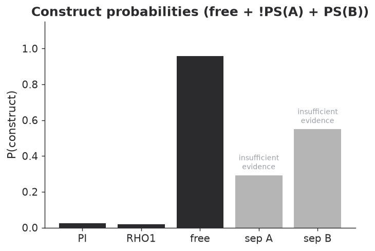

plot_diagnostics(fit, ci.counts)

plot_diagnostics(fit, cm)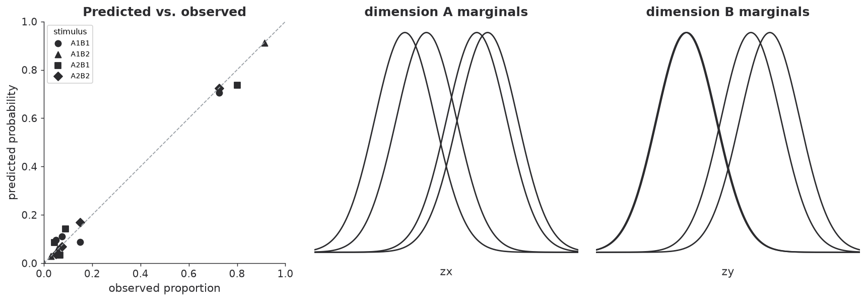

Read the diagnostics plot carefully. A poor reconstruction is a real warning, but a good one does not validate the GRT assumptions: the unconstrained model can reproduce any pattern of response proportions, so fitting well is not evidence that the model is right.

Do the whole sample

for pid, sub in trials.groupby("participant"):
    c = gt.to_confusion(sub, long=True,
                        factor_a=("a1", "a2"),
                        factor_b=("b1", "b2"), sep="/")
    _, cc = gt.infer(c.counts)
    print(pid, cc["p_PI"], cc["p_sep_A"])

for (pid in unique(trials$participant)) {
  sub <- trials[trials$participant == pid, ]
  c <- grin_to_confusion(sub, factor_a = c("a1","a2"),
                         factor_b = c("b1","b2"), sep = "/")
  f <- grin_infer(c$counts)
  cat(pid, f$constructs$p_PI, f$constructs$p_sep_A, "\n")
}

p01   p_PI = 0.024   p_sep_A = 0.292
p02   p_PI = 0.006   p_sep_A = 0.831
p03   p_PI = 0.059   p_sep_A = 0.831

In R, grin_tidy() returns one row per parameter per person, and the _group plotting functions take a list of fitted objects.

Know what the intervals mean

The interval on a marginal sensitivity means what it says. The interval on a within-stimulus correlation is narrower than nominal — across large held-out sets a 90% interval covers about 84% of the time. Both packages ship an optional correction, off by default:

fit, con = gt.infer(ci.counts, calibrated=True)
fit.std          # corrected widths
fit.std_raw      # what the network returned

fit <- grin_infer(ci$counts, calibrated = TRUE)
fit$result$std        # corrected widths
fit$result$std_raw    # what the network returned

Point estimates, construct probabilities and model selection are identical either way — only the stated uncertainty changes.